Manifold Constraint Hyperconnections

• Over the past decade there has been developments to residual connections in the form of hyper-connections.
• Hyper-connections increase the width of the residual streams while also increasing the diversity of patterns.
• Hyper-connections have increased performance gains but have adversely effected training stability, memory overhead and scalability.
• To overcome the challenges manifold-constraint hyper-connections (mHC) is introduced. It is a framework that projects the residual connection space of hyper-connections to a specific manifold to restore the identity matrix.
• The empirical experiments have proven that mHC are more effective for training at scale. mHC is seen as an extension of hyper-connections.

Introduction

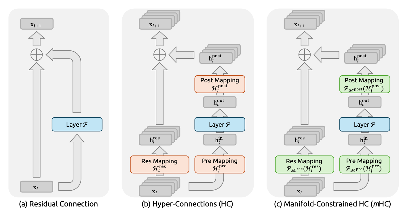
• Deep neural networks have gone through significant change in architecture as time has passed. ResNets were an important discovery that helped in promoting architectural performance. They are formulated as:

$x_{l+1} = x_l + \mathcal{F}(x_l, w_l)$

• Here $x_{l+1}$ and $x_l$ denote $C$ Dimensional input and output of the $x_l$ and $x_{l+1}$ layers. The function $\mathcal{F}$ is a residual function.
• The residual function has always been a part of architectural ideas. Ranging from attention to feed forward networks, it was always considered a key component.
• The residual connection paradigm always kept its original form throughout architectures. As attention became widely important in LLMs, so did residual connections.
• The success of residual connections were mainly attributed to its identity mapping property. This maintained stability during large scale training. By recursively incorporating the residual connection across multiple layers, the equation then becomes:

$x_L = x_l + \sum_{i=l}^{L-1} \mathcal{F}(x_i, w_i)$

• Here $x_L$ and $x_l$ refers to the outputs of the deeper and shallower layers. The identity mapping refers to the property that signal from the shallow layers maps directly onto the deeper layers.
• Recent studies have shown that hyper-connections, that is an extension of residual connections.
• Hyper-connections have expanded the width of the residual stream and enhancing complexity. Hyper-connections increase the topological complexity without increasing the overhead. Formally, a single layer propagation in hyper-connections is defined as:

$x_{l+1} = H_l^{res} x_l + H_l^{post} \mathcal{F}(H_l^{pre} x_l, w_l)$

Here $l$ denotes the layer, $H_l^{res}$ is a learnable mapping that mixes features within the residual stream. The $H_l^{pre}$ is a learnable mapping that converts the $nC$-dim stream into a $C$-dim stream. The $H_l^{post}$ does the opposite and maps the layer output back into the input.

• As the training scale increases, hyper-connections create instability and other issues. The primary concern is with the unrestricted nature of hyper-connections. In deeper architectures, identity mapping is a form of conservation mechanism. It makes sure that the average signal intensity across forward and backward passes are the same.
• Recursively using hyper-connections give us the following equation:

$x_L = \left( \prod_{i=1}^{L-l} H_{L-i}^{res} \right) x_l + \sum_{i=l}^{L-1} \left( \prod_{j=1}^{L-1-i} H_{L-j}^{res} \right) H_i^{post} \mathcal{F}(H_i^{pre} x_i, w_i)$

• The first learnable mapping is the cause of concern. It fails to maintain the global average. This leads to unbounded amplification or attenuation which causes instability during large scale training.
• Another issue is that even though hyper-connections increase efficiency in terms of FLOPs, there is no deeper investigation into memory access, particularly when the width of the residual stream is increased.
• Keeping all of this in mind, manifold-constraint hyper-connections (mHC) are introduced. It is a general framework that projects the residual connection space of the hyper-connections onto a manifold where the identity mapping can be restored.
• It also has vigorous infrastructure optimizations. Specifically, it uses the Sinkhorn-Knopp algorithm to project the $H^{res}$ onto a Birkhoff polytope.

Related Work

• Architectural advancements are mainly classified into 2 types:
  • a. Micro Design: Responsible for the design and architectural structure inside blocks.
  • b. Macro Design: Responsible for the global topology of the network.

Macro Design

• Driven by invariance and parameter sharing, convolutional architectures dominated. Later variations such as depth-wise convolution and grouped convolution increased efficiency.
• Transformers then ensured that attention and feed-forward neural networks became the fundamental architectural building blocks. Attention mechanisms were able to capture global information while FFNs (Feed-Forward Networks) enhanced the representational capacity of the individual features.

Macro Design

• Macro design governs the global topology of the network. Recently, macro-level design has shifted towards expanding the width of the residual stream. Hyper-connections introduced learnable matrices to modulate connection strength across various features.

Preliminary

• In hyper-connections, the input to the $l$-th layer $x_l \in \mathbb{R}^{n \times c}$ is expanded by a factor of '$n$' to construct a hidden matrix $x_l = (x_{l,0}^T, x_{l,1}^T, \dots, x_{l,n-1}^T)^T \in \mathbb{R}^{n \times c}$. This is viewed as an $n$-stream residual.
• This operation broadens the width of the residual stream.
• To govern the updating processes of the stream, HC introduces 3 learnable mappings: $H_l^{pre}, H_l^{post} \in \mathbb{R}^{1 \times n}$ and $H_l^{res} \in \mathbb{R}^{n \times n}$.
• In hyper-connections, learnable mappings are of 2 types: the input-dependent dynamic mapping and the global static mapping. The dynamic mappings are denoted by $\theta$ and the static mappings are denoted by the bias '$b$'.
• Formally, the HC formula is as follows:

$\tilde{x}_l = \text{RMSNorm}(x_l)$ $H_l^{pre} = \alpha_l^{pre} \cdot \tanh(\theta_l^{pre} \tilde{x}_l^T) + b_l^{pre}$ $H_l^{post} = \alpha_l^{post} \cdot \tanh(\theta_l^{post} \tilde{x}_l^T) + b_l^{post}$ $H_l^{res} = \alpha_l^{res} \cdot \tanh(\theta_l^{res} \tilde{x}_l^T) + b_l^{res},$

• RMSProp is only applied to the last dimension and $\alpha$ are scalar learnable gating factors assigned to small values.
• An interesting aspect is that the introduction of learnable mappings creates negligible computational overhead. This is because the expansion rate or value of $n$, which is typically 4, is insignificant when compared to the input dimension '$c$'.
• An ablation study of hyper-connections also shows us that $H^{res}$ leads to the most significant performance gain.

Numerical Instability

• While the $H^{res}$ learnable mapping is instrumental for performance, its sequential application possesses a significant risk. As stated earlier, HC is denoted by the following formula, in which $H^{res}$ is unconstrained. This mapping inevitably deviates from the identity mapping:

$x_L = \left( \prod_{i=1}^{L-l} H_{L-i}^{res} \right) x_l + \sum_{i=l}^{L-1} \left( \prod_{j=1}^{L-1-i} H_{L-j}^{res} \right) H_i^{post \top} \mathcal{F}(H_i^{pre} x_i, w_i),$

• As a result of this, the signal is prone to the exploding or vanishing gradients problem, which is what the residual connections are trying to solve.
• Empirical evidence also supports these claims, showing that during large-scale training around 12k steps, there is a loss surge.

System Overhead

• While the computational overhead of HC is manageable due to their linear mapping, the system-level overhead still remains a problem.
• Memory access I/O costs still pose a threat to modern architectural designs. This is often called the "memory wall".
• HC increases the memory access costs by a factor of '$n$'. This excessive I/O demand decreases training throughput.

Method	Operation	Read (Elements)	Write (Elements)
Residual Connection	Residual Merge	$2C$	$C$
	Total I/O	$2C$	$C$
Hyper-Connections	Calculate $H_l^{pre}, H_l^{post}, H_l^{res}$	$nC$	$n^2 + 2n$
	$H_l^{pre}$	$nC + n$	$C$
	$H_l^{post}$	$C + n$	$nC$
	$H_l^{res}$	$nC + n^2$	$nC$
	Residual Merge	$2nC$	$nC$
	Total I/O	$(5n+1)C + n^2 + 2n$	$(3n+1)C + n^2 + 2n$

Method

• Drawing inspiration from the identity mapping principle, the core idea of mHC is to constrain the residual mapping $H^{res}$ onto a specific manifold.
• The original identity mapping ensures stability by enforcing $H^{res} = I$.
• This is basically a method to prevent information exchange among the different streams.
• Projecting the mapping onto a manifold that simultaneously allows stability across layers while also allowing information exchange across streams.
• To enable this, $H^{res}$ is restricted to be a stochastic matrix (specifically, a doubly stochastic matrix), which is also called the Birkhoff polytope. Here, the matrix values are non-negative and sum up to 1.

$\mathcal{P}_{M^{res}}(H_l^{res}) := \{ H_l^{res} \in \mathbb{R}^{n \times n} \mid H_l^{res} \mathbf{1}_n = \mathbf{1}_n, \mathbf{1}_n^T H_l^{res} = \mathbf{1}_n^T, H_l^{res} \ge 0 \}$

• When $n=1$, the $H^{res}$ matrix becomes the scalar $1$.
• The choice for using the Birkhoff polytope comes from the following reasons:
  • a. Norm preservation: The spectral norm of a doubly stochastic matrix is $1$. This ensures the prevention of the vanishing gradients problem.
  • b. Composite closure: A set of doubly stochastic matrices are closed under matrix multiplication.
  • c. Geometric interpretation: The residual mapping acts as a convex combination of the permutations.

Parameterization and Manifold Projection

In this section, we detail the calculation process of $H_l^{pre}, H_l^{post}$, and $H_l^{res}$ in mHC. Given the input hidden matrix $x_l \in \mathbb{R}^{n \times C}$ at the $l$-th layer, we first flatten it into a vector $\tilde{x}_l = \text{vec}(x_l) \in \mathbb{R}^{1 \times nC}$ to preserve full context information. Then, we follow the original HC formulation to get the dynamic mappings and the static mappings as follows:

$$\begin{cases} \tilde{x}_l' = \text{RMSNorm}(\tilde{x}_l) \\ \tilde{H}_l^{pre} = \alpha_l^{pre} \cdot (\tilde{x}_l' \varphi_l^{pre}) + b_l^{pre} \\ \tilde{H}_l^{post} = \alpha_l^{post} \cdot (\tilde{x}_l' \varphi_l^{post}) + b_l^{post} \\ \tilde{H}_l^{res} = \alpha_l^{res} \cdot \text{mat}(\tilde{x}_l' \varphi_l^{res}) + b_l^{res}, \end{cases} \quad (7)$$

where $\varphi_l^{pre}, \varphi_l^{post} \in \mathbb{R}^{nC \times n}$ and $\varphi_l^{res} \in \mathbb{R}^{nC \times n^2}$ are linear projections for dynamic mappings and $\text{mat}(\cdot)$ is a reshape function from $\mathbb{R}^{1 \times n^2}$ to $\mathbb{R}^{n \times n}$.

Then, the final constrained mappings are obtained via:

$$\begin{cases} H_l^{pre} = \sigma(\tilde{H}_l^{pre}) \\ H_l^{post} = 2\sigma(\tilde{H}_l^{post}) \\ H_l^{res} = \text{Sinkhorn-Knopp}(\tilde{H}_l^{res}), \end{cases} \quad (8)$$

where $\sigma(\cdot)$ denotes the Sigmoid function. The Sinkhorn-Knopp$(\cdot)$ operator firstly makes all elements to be positive via an exponent operator and then conducts iterative normalization process that alternately rescales rows and columns to sum to 1. Specifically, given a positive matrix $\mathbf{M}^{(0)} = \exp(\tilde{H}_l^{res})$ as the start point, the normalization iteration proceeds as:

$\mathbf{M}^{(t)} = \mathcal{T}_r \left( \mathcal{T}_c(\mathbf{M}^{(t-1)}) \right), \quad (9)$

where $\mathcal{T}_r$ and $\mathcal{T}_c$ denote row and column normalization, respectively. This process converges to a doubly stochastic matrix $H_l^{res} = \mathbf{M}^{(t_{max})}$ as $t_{max} \to \infty$. We choose $t_{max} = 20$ as a practical value in our experiments.

Results

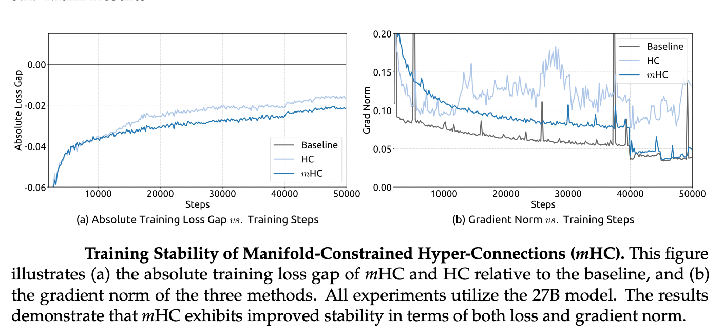
To evaluate the effectiveness of mHC, the researchers conducted large-scale training experiments using a 27B parameter model. They compared three configurations: a standard Baseline, unconstrained Hyper-Connections (HC), and our proposed Manifold-Constraint Hyper-Connections (mHC).

The results clearly indicate that while unconstrained hyper-connections offer potential, they introduce significant instability that mHC is uniquely designed to solve.

1. Absolute Training Loss Gap

The figure illustrates the absolute training loss gap relative to the baseline.

• The HC Struggle: While the unconstrained HC (light blue) initially tracks well, it exhibits a noisy and inconsistent loss profile. This volatility is a direct consequence of the "unrestricted nature" of hyper-connections mentioned in our earlier notes, which leads to signal deviation.

• The mHC Advantage: mHC (dark blue) not only remains stable but consistently maintains a lower loss than the baseline throughout the 50,000 steps. It achieves a final loss reduction of 0.021 compared to the baseline, proving that the manifold constraints allow the model to benefit from the expanded residual stream without the associated chaos.

2. Gradient Norm Analysis

The most compelling evidence for mHC’s stability is found in Figure 5(b), which tracks the Gradient Norm over training steps.

• Catastrophic Spikes: The unconstrained HC model suffers from massive, frequent spikes in gradient norm. These spikes represent the "unbounded amplification" risk we identified mathematically. In a production environment, these gradients often lead to "NaN" errors or total model collapse.

• Baseline-Level Stability: Remarkably, mHC exhibits a gradient profile that is almost as smooth as the standard baseline. By projecting Hres onto the Birkhoff polytope, we essentially "clamp" the spectral norm to 1. This ensures that even as the model complexity increases, the gradients remain well-behaved.

System-level Benchmark Results (27B Models)

The table below compares the performance of the Baseline, unconstrained Hyper-Connections (HC), and Manifold-Constraint Hyper-Connections (mHC) across 8 diverse downstream benchmarks. The experiments were conducted using 27B parameter models to test effectiveness in large-scale pre-training.

Benchmark (Metric)	BBH (EM)	DROP (F1)	GSM8K (EM)	HellaSwag (Acc.)	MATH (EM)	MMLU (Acc.)	PIQA (Acc.)	TriviaQA (EM)
# Shots	3-shot	3-shot	8-shot	10-shot	4-shot	5-shot	0-shot	5-shot
27B Baseline	43.8	47.0	46.7	73.7	22.0	59.0	78.5	54.3
27B w/ HC	48.9	51.6	53.2	74.3	26.4	63.0	79.9	56.3
27B w/ mHC	51.0	53.9	53.8	74.7	26.0	63.4	80.5	57.6

Analysis of Downstream Performance

The benchmark results solidify mHC as the superior architecture for scaling. While the transition from standard residual connections to unconstrained hyper-connections (HC) provides a significant jump in performance, it is the addition of the manifold constraint that truly unlocks the model's potential:

• Consistency is Key: mHC outperforms the baseline on every single benchmark and surpasses the unconstrained HC on 7 out of 8 tests.
• Reasoning & Math: In complex reasoning tasks like BBH and GSM8K, mHC shows a massive improvement over the baseline (e.g., a +7.1% jump in GSM8K), proving that broader residual streams enhance the model's "thinking" depth.
• The Robustness of mHC: Even in cases where HC was competitive (like the MATH benchmark), mHC remains within a negligible margin while providing the training stability that unconstrained HC lacks.

Scaling Experiments

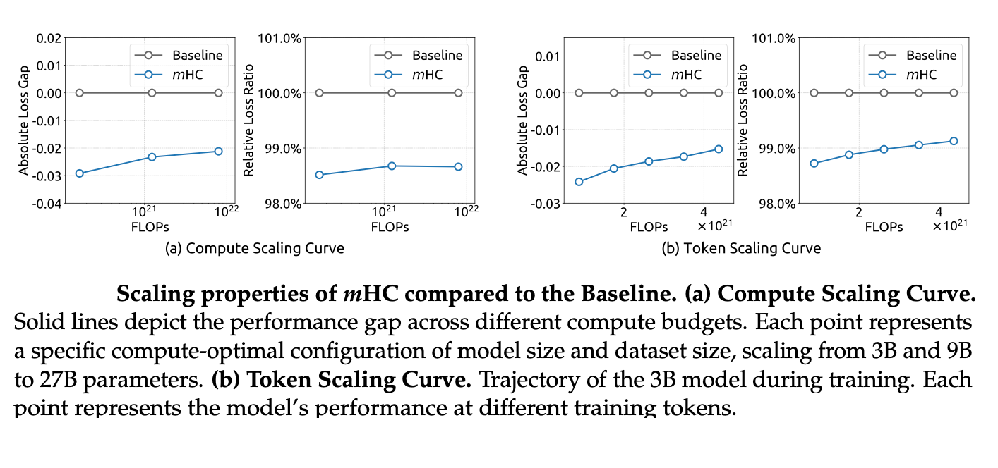
The figure illustrates the scaling properties of mHC compared to the Baseline across various compute budgets and training durations. The results highlight the consistent efficiency of manifold-constrained architectures as resource allocation increases.

(a) Compute Scaling Curve

• Solid lines depict the performance gap across different compute budgets.
• Each data point represents a specific compute-optimal configuration of model size and dataset size, scaling from 3B to 9B and 27B parameters.
• The Absolute Loss Gap remains consistently negative (below the baseline), indicating that mHC yields better performance than standard architectures at every tested scale.

(b) Token Scaling Curve

• This shows the trajectory of the 3B model during the training process.
• Each point represents the model's performance at different counts of training tokens.
• The Relative Loss Ratio demonstrates that mHC maintains a significant performance advantage (approximately 1-2% better) throughout the entire training duration, rather than just at the end.

Summary of Scaling Benefits:

• Efficiency: mHC models achieve lower loss for the same amount of floating-point operations (FLOPs) compared to baselines.
• Predictability: The scaling curves for mHC are smooth and consistent, suggesting that benefits observed at smaller scales (3B) reliably translate to larger scales (27B).

References

• [1] Xie, Z., Wei, Y., Cao, H., et al. (2026). mHC: Manifold-Constrained Hyper-Connections. arXiv preprint arXiv:2512.24880v2 [cs.CL]. [Online]. Available: https://arxiv.org/abs/2512.24880