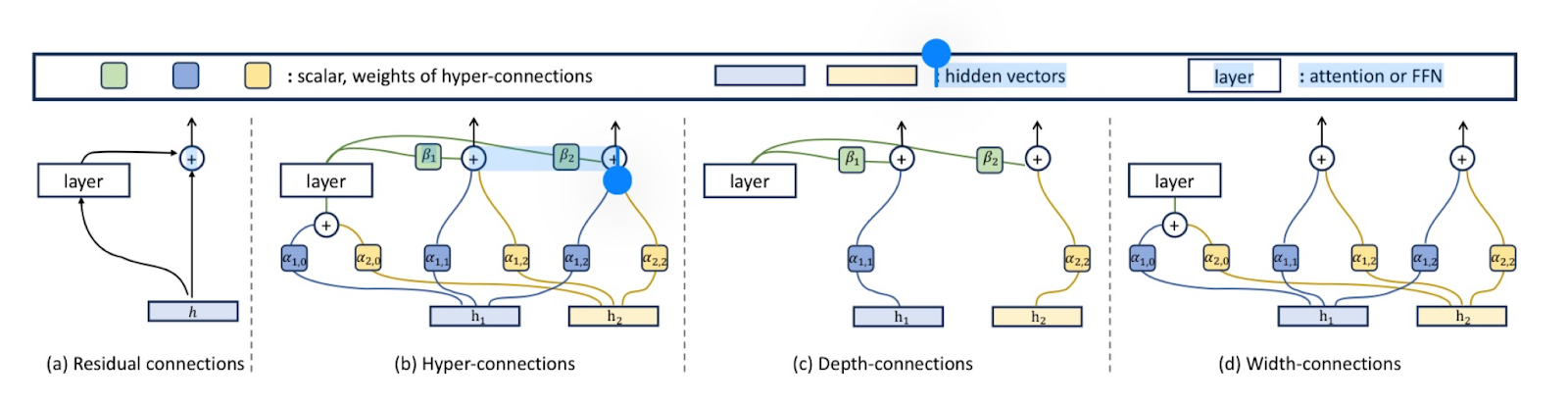
• Hyper-connections are introduced as an alternative to residual connections. This addresses the "seesaw effect" caused by the trade-off between vanishing gradients and representation collapse. Theoretically, hyper-connections allow the network to control the strength of connections at features of different depths and dynamically rearrange layers.

Introduction

• Deep learning has had immense success with residual connections in various domains, including CNNs and Transformers.
• Residual connections help reduce the vanishing gradient problem, though they are not an infallible solution.
• The two main variants of residual connections are:
  • Pre-Norm: Normalization is applied before the residual block. This mitigates vanishing gradients but introduces representation collapse, where deeper layers become extremely similar.
  • Post-Norm: Normalization happens after the residual block. This mitigates representation collapse but reintroduces the vanishing gradient issue.
• Balancing these two issues is like a "seesaw" because these variants predefine the fixed strength of the output and input within the layer.

• Driven by these limitations, the authors explored whether a network can autonomously learn the optimal strength of connections to improve performance.
• Hyper-connections achieve this, improving performance with almost negligible increases in computation and parameters.
• The core idea is to propose learnable depth and width connections, flexibly integrating features vertically across depths compared to standard residual connections.
• Depth connections act as generalized residual connections, assigning weights to the links between input and output.
• To model different depth connections simultaneously, the input is expanded into $n$ copies, each with its own depth connection. This allows multiple hidden vectors to preserve various patterns from preceding layers.
• Width connections exist between these $n$ hidden vectors, allowing information exchange within the same layer.
• Experiments suggest that $n > 1$ is required for performance improvements; with $n = 1$, the seesaw effect persists.
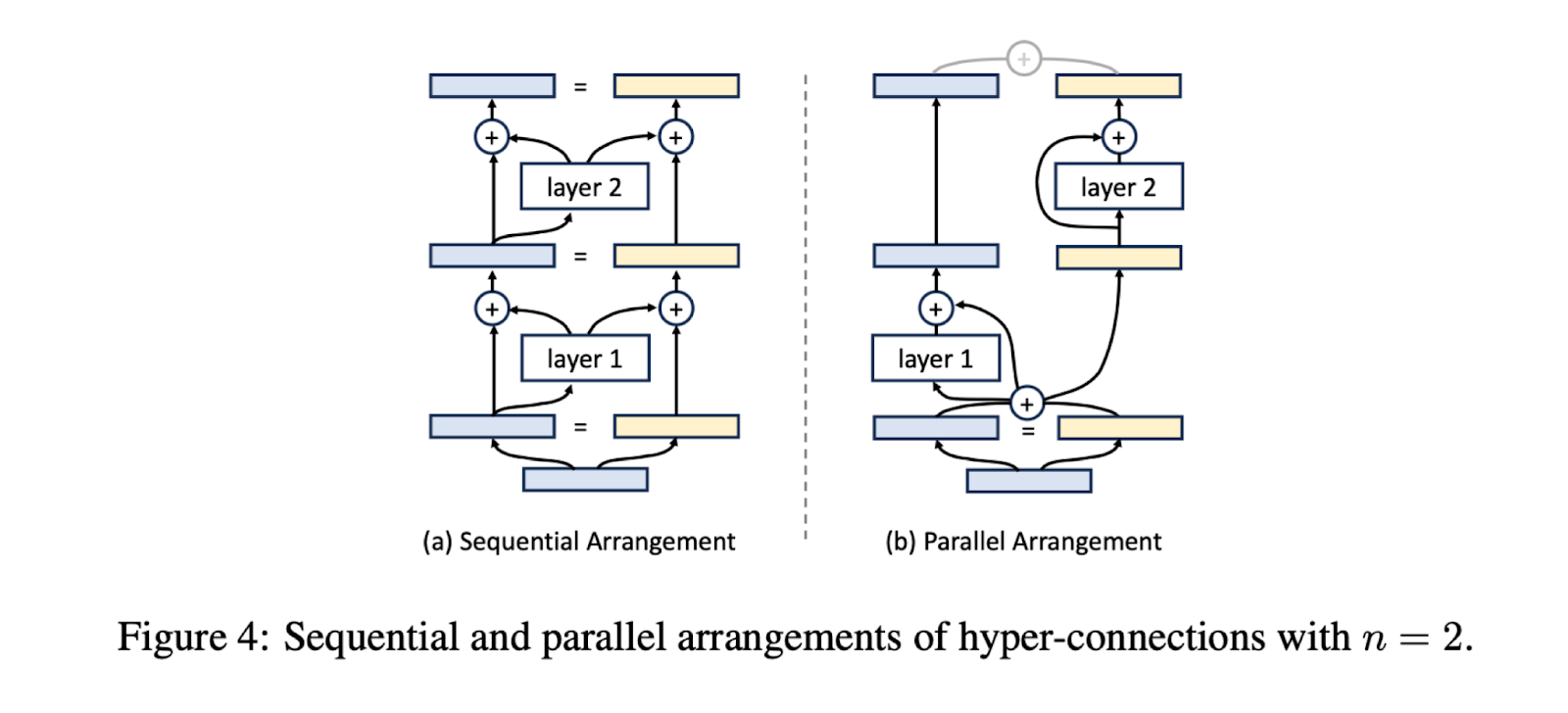
• When $n > 1$, hyper-connections can learn to adjust residual strength and rearrange layers both sequentially and in parallel.
• Dynamic Hyper Connections (DHC) further enhance flexibility by enabling the network to adjust connection weights based on the input.
• Despite the width increasing $n$ times, the computational costs remain almost negligible.
• While primary research focused on LLMs, the benefits extend to image generation and classification tasks.
• Using Pre-Norm as a baseline, hyper-connections show benefits across 1B, 7B dense models, and 70B MoE models.
• Models using hyper-connections converge 1.8 times faster and maintain lower feature similarity across adjacent layers.

Method

• Consider the hidden vector $h^{k-1}$ for the $k^{th}$ layer. It has an initial input vector called $h^0$ which is the initial hidden vector for the layer.
• $h^0$ is repeated '$n$' times to get a hyper hidden matrix. This is denoted by $\mathcal{H}^0 = (h^0, h^0, h^0 \dots h^0)^T$.
• The variable '$n$' is called the expansion rate.
• For the $k^{th}$ layer, it contains the hyper hidden matrix of the $(k-1)^{th}$ layer. It is denoted as $\mathcal{H}^{k-1} = (h^{k-1}, h^{k-1}, h^{k-1} \dots h^{k-1})^T$.
• Finally, the sum of rows of the last hyper hidden matrix is taken to obtain the hidden vector, which is then passed through a projection layer so that it produces the output of the network.
• The hyper connections can be denoted as a matrix $\mathcal{HC}$ where each element is a connection weight.
• The matrix is made of 3 smaller matrices: $\mathbf{A_m}$, $\mathbf{A_r}$, and $\mathbf{B}$.
• The matrix is denoted as:

$\mathcal{HC} = \begin{pmatrix} \mathbf{0}_{1 \times 1} & \mathbf{B} \\ \mathbf{A_m} & \mathbf{A_r} \end{pmatrix} = \begin{pmatrix} 0 & \beta_1 & \beta_2 & \cdots & \beta_n \\ \alpha_{1,0} & \alpha_{1,1} & \alpha_{1,2} & \cdots & \alpha_{1,n} \\ \alpha_{2,0} & \alpha_{2,1} & \alpha_{2,2} & \cdots & \alpha_{2,n} \\ \vdots & \vdots & \vdots & \ddots & \vdots \\ \alpha_{n,0} & \alpha_{n,1} & \alpha_{n,2} & \cdots & \alpha_{n,n} \end{pmatrix} \in \mathbb{R}^{(n+1) \times (n+1)}.$

• Consider a network layer $T$. The output of $\mathcal{HC}$ is denoted by $\hat{H}$ and is formulated as:

$\hat{H} = \mathcal{HC}(T, H) = \mathbf{B}^T T(H^T \mathbf{A_m})^T + \mathbf{A_r}^T H$

• $\mathbf{A_m}$ is used as a weighted sum of the input $H = (h_1, h_2, h_3 \dots h_n)^T$ to obtain the input $h_0^T$ of the current network layer $T$:

$h_0^T = \mathbf{A_m}^T H$

• $\mathbf{A_r}$ is used to connect $H$ and map it to the hyper hidden matrix:

$H' = \mathbf{A_r}^T H$

• The 2 types of hyper connections are denoted as:
  • a. Depth wise: $\mathcal{DC} = \begin{pmatrix} \mathbf{B} \\ \text{diag}(\mathbf{A_r}) \end{pmatrix} = \begin{pmatrix} \beta_1 & \beta_2 & \cdots & \beta_n \\ \alpha_{1,1} & \alpha_{2,2} & \cdots & \alpha_{n,n} \end{pmatrix} \in \mathbb{R}^{2 \times n}$
  • b. Width wise: $\mathcal{WC} = (\mathbf{A_m} \quad \mathbf{A_r}) \in \mathbb{R}^{n \times (n+1)}$

Dynamic Hyper Connections

• The entries of $\mathcal{HC}$ can dynamically depend on the input $H$. The matrix representation of this is as follows:

$\mathcal{HC}(\mathbf{H}) = \begin{pmatrix} \mathbf{0}_{1 \times 1} & \mathbf{B}(\mathbf{H}) \\ \mathbf{A_m}(\mathbf{H}) & \mathbf{A_r}(\mathbf{H}) \end{pmatrix}$

• In practice, we combine both dynamic and static matrices to achieve DHC. The dynamic parameters are obtained through linear transformation of the input $H$.
• To stabilize the training process, normalization is done and then tanh activation is done:

$\overline{\mathbf{H}} = \text{norm}(\mathbf{H})$ $\mathcal{B}(\mathbf{H}) = s_\beta \circ \tanh(\overline{\mathbf{H}}\mathbf{W}_\beta)^T + \mathbf{B} \in \mathbb{R}^{1 \times n}$ $\mathcal{A}_m(\mathbf{H}) = s_\alpha \circ \tanh(\overline{\mathbf{H}}\mathbf{W}_m) + \mathbf{A}_m \in \mathbb{R}^{n \times 1}$ $\mathcal{A}_r(\mathbf{H}) = s_\alpha \circ \tanh(\overline{\mathbf{H}}\mathbf{W}_r) + \mathbf{A}_r \in \mathbb{R}^{n \times n}$

---

Initialization

• In order to make the initializations the same as pre-norm residual connections, the $w_\beta, w_m$ and $w_r$ in the above equation are set to zero.
• The static matrices are defined as follows:

$\begin{pmatrix} \mathbf{0}_{1 \times 1} & \mathbf{B}^k \\ \mathbf{A}_m^k & \mathbf{A}_r^k \end{pmatrix} = \begin{pmatrix} 0_{1 \times 1} & \mathbf{1}_{1 \times n} \\ e_{k \pmod n} & e_{n \times n} \end{pmatrix}$

where $k$ is the index of the layer and \pmod denotes the modulo operation.

Why Hyper Connections

• They explore how hyper connection in their non-trainable form represent pre-norm and post-norm architectures.
• The concept of sequential-parallel duality is introduced so that it can be visualized how hyper connections can dynamically optimize layer arrangement to enhance network performance.
• Pre-norm and post-norm connections can be represented as the following hyperconnection matrices with the expansion rate $n=1$:

$HC_{PreNorm} = \begin{pmatrix} 0 & 1 \\ 1 & 1 \end{pmatrix}, \quad \quad HC_{PostNorm} = \begin{pmatrix} 0 & \frac{1}{\sqrt{\sigma_i^2 + \sigma_o^2 + 2\sigma_{io}}} \\ 1 & \frac{1}{\sqrt{\sigma_i^2 + \sigma_o^2 + 2\sigma_{io}}} \end{pmatrix}$

• $\sigma_i$ and $\sigma_o$ are the standard deviations of the input and output layers. The covariance between these are represented as $\sigma_{io}$.

• For pre-norm, the hyper connection matrix is a $2 \times 2$ matrix, with $1$s on the right lower upper triangle part and the rest have a placeholder value of zero in them.

• For post-norm, the weights depend on the co-variance and variances of the input and output layer. This gives us a $2 \times 2$ non-trainable matrix.

• Hyper connections give us a $(n+1) \times (n+1)$ trainable matrix.

• Given a series of neural networks, we have the option to arrange them either sequentially or in parallel. Hyper-connections make it possible to blend both of these configurations into one.

Result table

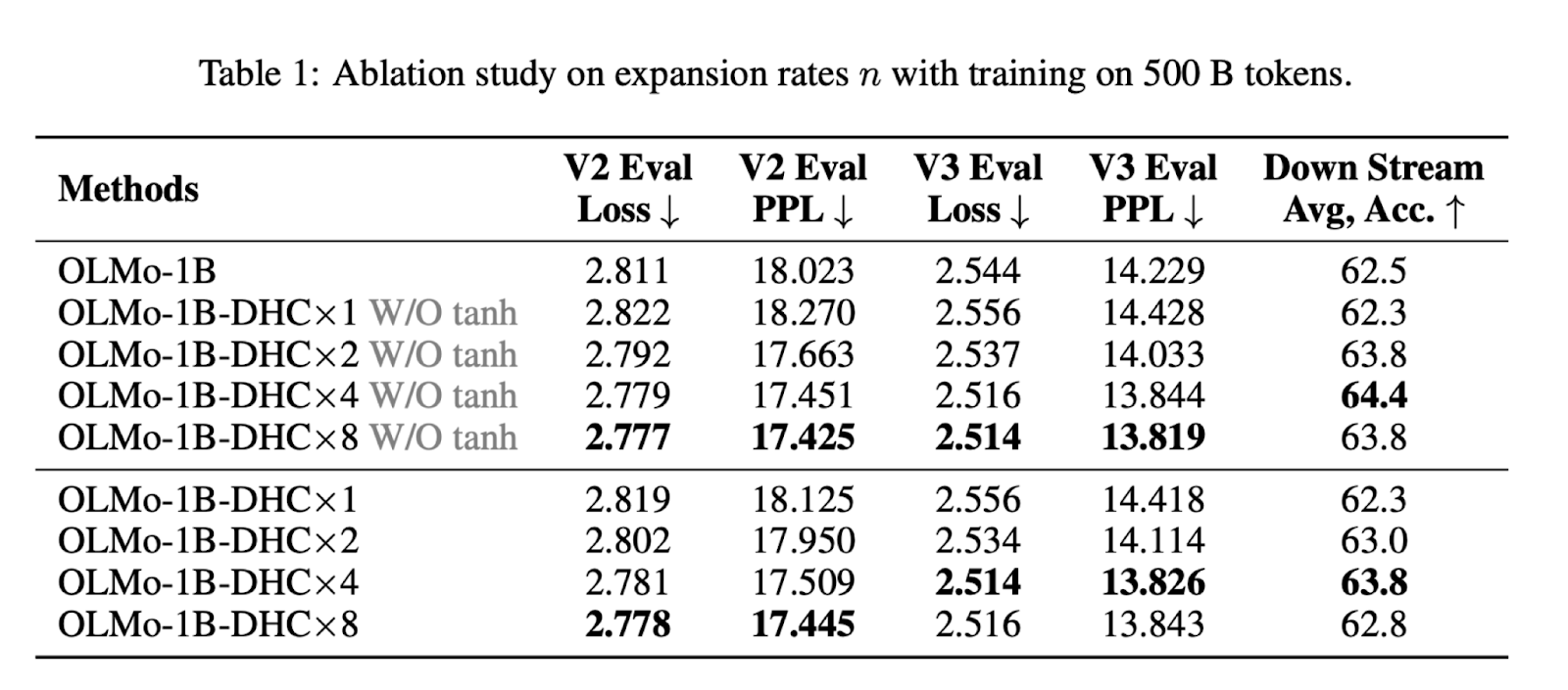
• Based on the results, increasing the expansion rate n generally improves model performance by reducing evaluation loss and perplexity (PPL) across both V2 and V3 datasets, with the OLMo-1B-DHC $\times$ 8 configurations consistently achieving the lowest loss and PPL values.

References

1. Zhu, D., Huang, H., Huang, Z., Zeng, Y., Mao, Y., Wu, B., Min, Q., & Zhou, X. (2024). Hyper-Connections. arXiv preprint arXiv:2409.19606.

2. He, K., Zhang, X., Ren, S., & Sun, J. (2016). Deep Residual Learning for Image Recognition. In Proceedings of the IEEE Conference on Computer Vision and Pattern Recognition (CVPR). arXiv:1512.03385.